Using Amazon RedShift with the AWS .NET API Part 7: data warehousing and the star schema

Introduction

In the previous post we dived into Postgresql statement execution on a RedShift cluster using C# and ODBC. We saw how to execute a single statement or many of them at once. We also tested a parameterised query which can protect us from SQL injections.

In this post we’ll deviate from .NET a little and concentrate on the basics of data warehousing and data mining in RedShift. In particular we’ll learn about a popular schema type often used in conjunction with data mining: the star schema.

Star and snowflake schemas

I went through the basic characteristics of star and snowflake schemas elsewhere on this blog, I’ll copy the relevant parts here.

Data warehousing requires a different mindset to what you might be accustomed to from your DB-driven development experience. In a “normal” database of a web app you’ll probably have tables according to your domain like “Customer”, “Product”, “Order” etc. Then you’ll have secondary keys and intermediate tables to represent 1-to-M and M-to-M relationships. Also, you’ll probably keep your tables normalised.

That’s often simply not good enough for analytic and data mining applications. In data analysis apps your customers will be after some complex aggregation queries:

• What was the maximum response time of /Products.aspx on my web page for users in Seattle using IE 10 on January 12 2015?
• What was the average sales of product ‘ABC’ in our physical shops in the North-America region between 01 and 20 December 2014?
• What is the total value of product XYZ sold on our web shop from iOS mobile apps in France in February 2015 after running a campaign?

You can replace “average” and “maximum” with any other aggregation type such as the 95th-percentile and median. With so many aggregation combinations your aggregation scripts would need to go through a very long list of aggregations. Also, trying to save every thinkable aggregation combination in different tables would cause the number of tables to explode. Such a setup will require a lot of lookups and joins which greatly reduce the performance. We haven’t even mentioned the difficulty with adding new aggregation types and storing historical data.

Data mining applications have adopted two schema types specially designed to solve this problem:

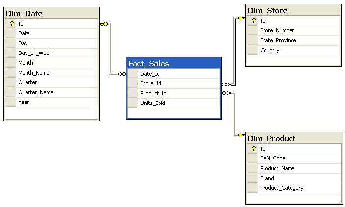
• Star schema: a design with a Fact table in the middle and one or more Dimension tables around. The dimension tables are often denormalised
• Snowflake schema: very similar to a star schema but the dimension tables are normalised. Therefore the fact table is surrounded by the dimension tables and their own broken-out sub-tables

Here’s an example for each type from Wikipedia to give you a taste.

Star:

Snowflake:

They are often used by analytic applications such as SQL Server Analysis Services. If you’re planning to take on data mining at a serious level then it’s inevitable to get accustomed with them.

There’s long article that goes through Star and Snowflake in RedShift available here.

Our goals

Our main goal is to extend our URL response time model a bit and build a very simple star schema. It will be very basic but if you’re new to this stuff then it’s for the better.

We’ll keep our basic concept of URL response times but add one more property: the customer name. If you’ve followed through the series on Big Data on this blog then this will sound familiar.

Our intention is to aggregate the URL response times by URL and Customer. This means that we’ll have two dimensions in the star schema: the URL dimension and the Customer dimension. We’ll include the following aggregations by each dimension:

• The average, min and max response time for a given URL and Customer combination
• The total number of URLs for a given URL and Customer combination
• The median, 95th and 99th percentile of the response time for a given URL and Customer combination

In the remainder of this post we’ll build the necessary table for our minimised data warehousing scenario.

Create a RedShift cluster in code or via the GUI like we saw before or reuse an existing one. Connect to the master node with WorkbenchJ and get ready to write some Postgresql.

Building the raw data table

The raw data table will be the same as before but we add a customer_name column:

DROP TABLE IF EXISTS url_response_times;
CREATE TABLE url_response_times (url varchar, customer_name varchar, response_time int);

We imagine in this scenario that we measure the response times of our own web site which is used by different customers. Execute the following INSERT statements to fill the url_response_times table with the records:

INSERT INTO url_response_times VALUES ('www.mysite.com/home', 'Favourite customer', 354);
INSERT INTO url_response_times VALUES ('www.mysite.com/history', 'Favourite customer', 735);
INSERT INTO url_response_times VALUES ('www.mysite.com/plans','Favourite customer',1532);
INSERT INTO url_response_times VALUES ('www.mysite.com/home','Favourite customer',476);
INSERT INTO url_response_times VALUES ('www.mysite.com/history','Favourite customer',1764);
INSERT INTO url_response_times VALUES ('www.mysite.com/plans','Favourite customer',1467);
INSERT INTO url_response_times VALUES ('www.mysite.com/home','Favourite customer',745);
INSERT INTO url_response_times VALUES ('www.mysite.com/history','Favourite customer',814);
INSERT INTO url_response_times VALUES ('www.mysite.com/plans','Favourite customer',812);
INSERT INTO url_response_times VALUES ('www.mysite.com/home','Nice customer',946);
INSERT INTO url_response_times VALUES ('www.mysite.com/history','Nice customer',1536);
INSERT INTO url_response_times VALUES ('www.mysite.com/plans','Nice customer',2643);
INSERT INTO url_response_times VALUES ('www.mysite.com/home','Nice customer',823);
INSERT INTO url_response_times VALUES ('www.mysite.com/history','Nice customer',1789);
INSERT INTO url_response_times VALUES ('www.mysite.com/plans','Nice customer',967);
INSERT INTO url_response_times VALUES ('www.mysite.com/home','Nice customer',1937);
INSERT INTO url_response_times VALUES ('www.mysite.com/history','Nice customer',3256);
INSERT INTO url_response_times VALUES ('www.mysite.com/plans','Nice customer',2547);

OK, let’s move on.

Building the dimension tables

The next step is to build the 2 dimension tables DimUrl and DimCustomer. Both tables will have a column called ‘dw_id’ which stands for data warehouse id. Another common column is the insertion date.

Execute the following code to create DimUrl:

DROP TABLE IF EXISTS DimUrl CASCADE;
CREATE TABLE DimUrl
(
		dw_id            integer         NOT NULL,
		url varchar NOT NULL,
		inserted_utc     timestamp       default convert_timezone('CET','UTC', getdate()) NOT NULL
);

ALTER TABLE DimUrl
   ADD CONSTRAINT DimUrl_pkey
   PRIMARY KEY (dw_id);

COMMIT;

The RedShift version of Postgresql doesn’t allow us to create auto-incrementing primary keys, We’ll see a trick in the next post how to make the IDs unique. I haven’t found any simple way to insert the UTC date in RedShift so I had to use the convert_timezone function which converts my current timezone “CET” into UTC. The getdate() function simply returns the current date in the timezone of the machine without the timezone information. So you’ll probably need to modify the code to reflect your timezone. If you have a simpler way of achieving the same then you’re welcome to present it in the comments section.

We then turn dw_id into the primary key of the table and commit the changes.

The code to create DimCustomer is almost identical:

DROP TABLE IF EXISTS DimCustomer CASCADE;
CREATE TABLE DimCustomer
(
		dw_id            integer         NOT NULL,
		name varchar not null,
		inserted_utc     timestamp       default convert_timezone('CET','UTC', getdate()) NOT NULL
);

ALTER TABLE DimCustomer
   ADD CONSTRAINT DimCustomer_pkey
   PRIMARY KEY (dw_id);

COMMIT;

Building the fact table

The fact table will reference our dimension tables and store the aggregations for each combination of Url and Customer. You can imagine that the fact table can grow a lot larger with other dimensions: location, browser type, etc.

DROP TABLE IF EXISTS FactAggregationUrl CASCADE;
CREATE TABLE FactAggregationUrl
(
	url_id int NOT NULL references dimurl(dw_id),
	customer_id int NOT NULL references dimcustomer(dw_id),	
	url_call_count int not null,
	min int NOT NULL,
	max int NOT NULL,
	avg double precision NOT NULL,
	median double precision NOT NULL,
	percentile_95 double precision NOT NULL,
	percentile_99 double precision NOT NULL,
	inserted_utc     timestamp       default convert_timezone('CET','UTC', getdate()) NOT NULL
);

COMMIT;

We’ll continue with this scenario in the next post.

View all posts related to Amazon Web Services and Big Data here.