Using Amazon RedShift with the AWS .NET API Part 9: data warehousing and the star schema 3

Introduction

In the previous post we started formulating a couple of Postgresql statements to fill in the dimension tables and the aggregation values. We saw that it wasn’t particularly difficult to calculate some basic aggregations over combinations of URL and Customer. We ignored the calculation of the median and percentile values and set them to 0. I’ve decided to dedicate a post just for those functions as I thought they were a lot more complex than min, max and average.

Median in RedShift

Median is also a percentile value, it is the 50th percentile. So we could use the percentile function for the median as well but median has its own dedicated function in RedShift. It’s not a compact function, like min() where you can pass in one or more arguments and you get a single value.

Let’s try and use the function to calculate the median over all values we currently have in url_response_times:

select median(response_time) over() from url_response_times;

The function will return 1217 for every row in the data set:

We can have a single value using the distinct keyword:

select distinct(median) from(select median(response_time) over() from url_response_times);

That gives 1217 which is the correct value for the full data set. However, that’s not really what we need. We’d like to see the median response time by URL and Customer. The following extended statement does the trick with the help of the PARTITION BY and GROUP BY clauses:

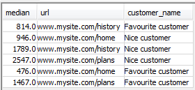
select distinct median
			(response_time)
		over (partition by url, customer_name) as median, url,customer_name from url_response_times
		group by 
			(response_time)
			, url, customer_name;

We now have the correct figures:

However, how do we add all that into our aggregation script? We need to turn the above function into a subset and reference it from the encasing script. We also need to extend the WHERE and GROUP BY clauses to take this subset into consideration:

select
	u.dw_id as url_id		
	, c.dw_id as customer_id
	, count(u.dw_id) as url_count
	, MIN(response_time) as min_response_time
	, MAX(response_time) as max_response_time
	, AVG(response_time) as avg_response_time
	,median as med
	,0 as perc_95
	,0 as perc_99
from
	url_response_times d,	
  DimUrl u,  
  DimCustomer c,
  (select distinct median
			(response_time)
		over (partition by url, customer_name) as median, url,customer_name from url_response_times
		group by 
			(response_time)
			, url, customer_name) med
where	
  d.url = u.url 
  	and d.customer_name = c.name			
  	and d.url = med.url
  	and d.customer_name = med.customer_name
group by 
	u.dw_id	
	, c.dw_id
	, med.median;

Let’s see what we have now:

Percentiles in RedShift

We need to go through a similar process with the percentiles as the RedShift percentile_cont is a window function with a couple of clauses on its own. The following statement will return the 95th percentile for each record in the table:

select perc from (select (response_time), percentile_cont (0.95) within group (order by (response_time)) over () as perc from url_response_times);

Like above we can have a single value using the distinct keyword:

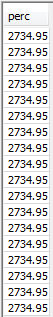
select distinct(perc) from(select perc from (select (response_time), percentile_cont (0.95) within group (order by (response_time)) over () as perc from url_response_times));

…which returns 2734.95. Let’s see what this function will look like to view the percentiles by URL and Customer:

select distinct(percentile_95) AS percentile_95, url,customer_name from (select (response_time), percentile_cont (0.95) within group (order by (response_time)) over (partition by url, customer_name) as percentile_95, url, customer_name from url_response_times group by response_time, url, customer_name);

…which gives the correct aggregations:

The 99th percentile calculation will be the same, we just need to pass 0.99 into the percentile_cont function.

Let’s turn this statement into a derived table and finalise our aggregation script:

select
	u.dw_id as url_id		
	, c.dw_id as customer_id
	, count(u.dw_id) as url_count
	, MIN(response_time) as min_response_time
	, MAX(response_time) as max_response_time
	, AVG(response_time) as avg_response_time
	,median as med
	,percentile_95 as perc_95
	,percentile_99 as perc_99
from
	url_response_times d,	
  DimUrl u,  
  DimCustomer c,
  (select distinct median
			(response_time)
		over (partition by url, customer_name) as median, url,customer_name from url_response_times
		group by 
			(response_time)
			, url, customer_name) med,
	 (select distinct(percentile_95) AS percentile_95, url,customer_name from (select (response_time), 
	 		percentile_cont (0.95) within group (order by (response_time)) 
	 		over (partition by url, customer_name) as percentile_95, url, customer_name from url_response_times group by response_time, url, customer_name)) perc_95,
	 (select distinct(percentile_99) AS percentile_99, url,customer_name from (select (response_time), 
	 		percentile_cont (0.99) within group (order by (response_time)) 
	 		over (partition by url, customer_name) as percentile_99, url, customer_name from url_response_times group by response_time, url, customer_name)) perc_99	
where	
  d.url = u.url 
  	and d.customer_name = c.name			
  	and d.url = med.url
  	and d.customer_name = med.customer_name
  	and d.url = perc_95.url
  	and d.customer_name = perc_95.customer_name
  	and d.url = perc_99.url
  	and d.customer_name = perc_99.customer_name
group by 
	u.dw_id	
	, c.dw_id
	, med.median
	, perc_95.percentile_95
	, perc_99.percentile_99;

…and we have the correct calculations in place now:

Completing the fact table insertions

The last step now is to add these aggregated values to our fact table. That’s quite trivial:

insert into FactAggregationUrl
(
	url_id,
	customer_id,	
	url_call_count,
	min,
	max,
	avg,
	median,
	percentile_95,
	percentile_99
)
select
	u.dw_id	
	, c.dw_id
	, count(u.dw_id)
	, MIN(response_time)
	, MAX(response_time)
	, AVG(response_time)
	,median
	,percentile_95
	,percentile_99
from
	url_response_times d,	
  DimUrl u,  
  DimCustomer c,
  (select distinct median
			(response_time)
		over (partition by url, customer_name) as median, url,customer_name from url_response_times
		group by 
			(response_time)
			, url, customer_name) med,
	 (select distinct(percentile_95) AS percentile_95, url,customer_name from (select (response_time), 
	 		percentile_cont (0.95) within group (order by (response_time)) 
	 		over (partition by url, customer_name) as percentile_95, url, customer_name from url_response_times group by response_time, url, customer_name)) perc_95,
	 (select distinct(percentile_99) AS percentile_99, url,customer_name from (select (response_time), 
	 		percentile_cont (0.99) within group (order by (response_time)) 
	 		over (partition by url, customer_name) as percentile_99, url, customer_name from url_response_times group by response_time, url, customer_name)) perc_99	
where	
  d.url = u.url 
  	and d.customer_name = c.name			
  	and d.url = med.url
  	and d.customer_name = med.customer_name
  	and d.url = perc_95.url
  	and d.customer_name = perc_95.customer_name
  	and d.url = perc_99.url
  	and d.customer_name = perc_99.customer_name
group by 
	u.dw_id	
	, c.dw_id
	, med.median
	, perc_95.percentile_95
	, perc_99.percentile_99;

Let’s check the contents of the fact table:

select * from factaggregationurl;

Great, we have fulfilled all aggregation goals we set out before.

This was the last post of the actual series on RedShift. The next post will look at the larger picture and discuss RedShift’s place in Big Data. We’ll put RedShift to work in the overall Big Data demo application we started building way back in the first post on Amazon Kinesis.

View all posts related to Amazon Web Services and Big Data here.